[Presentation Title]


Problem and opportunity: Big, dynamic data
- Electrophysiology ⇒ Optogenetics
- Calcium-sensitive fluorescent proteins
- Voltage-sensitive fluorescent proteins
- In vivo recording with mini-microscopes
- Electroencephalography (EEG)
- Magnetoencephalography (MEG)
- Functional Magnetic Resonance Imaging (fMRI)
Examples with multi-electrode arrays
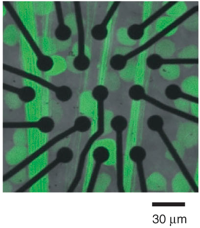
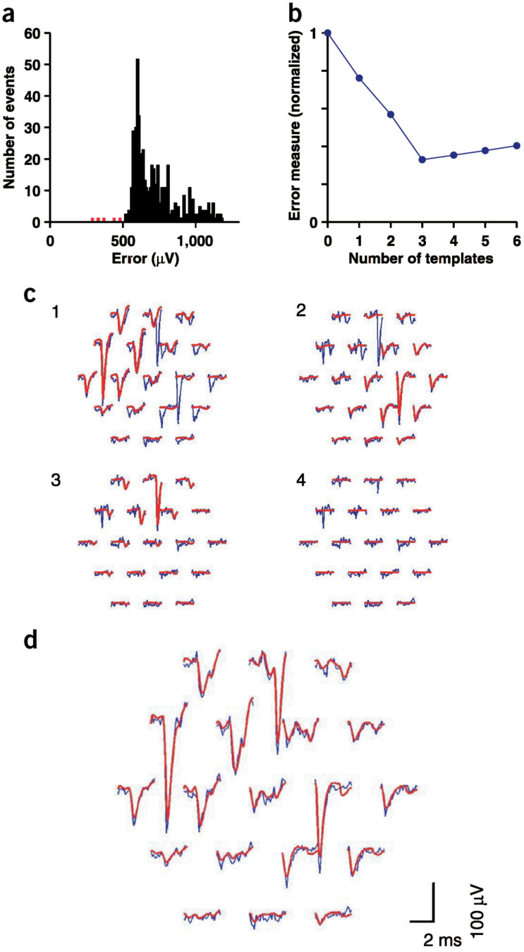
Marre et al, J. Neurosci. 32, 14859 (2012)
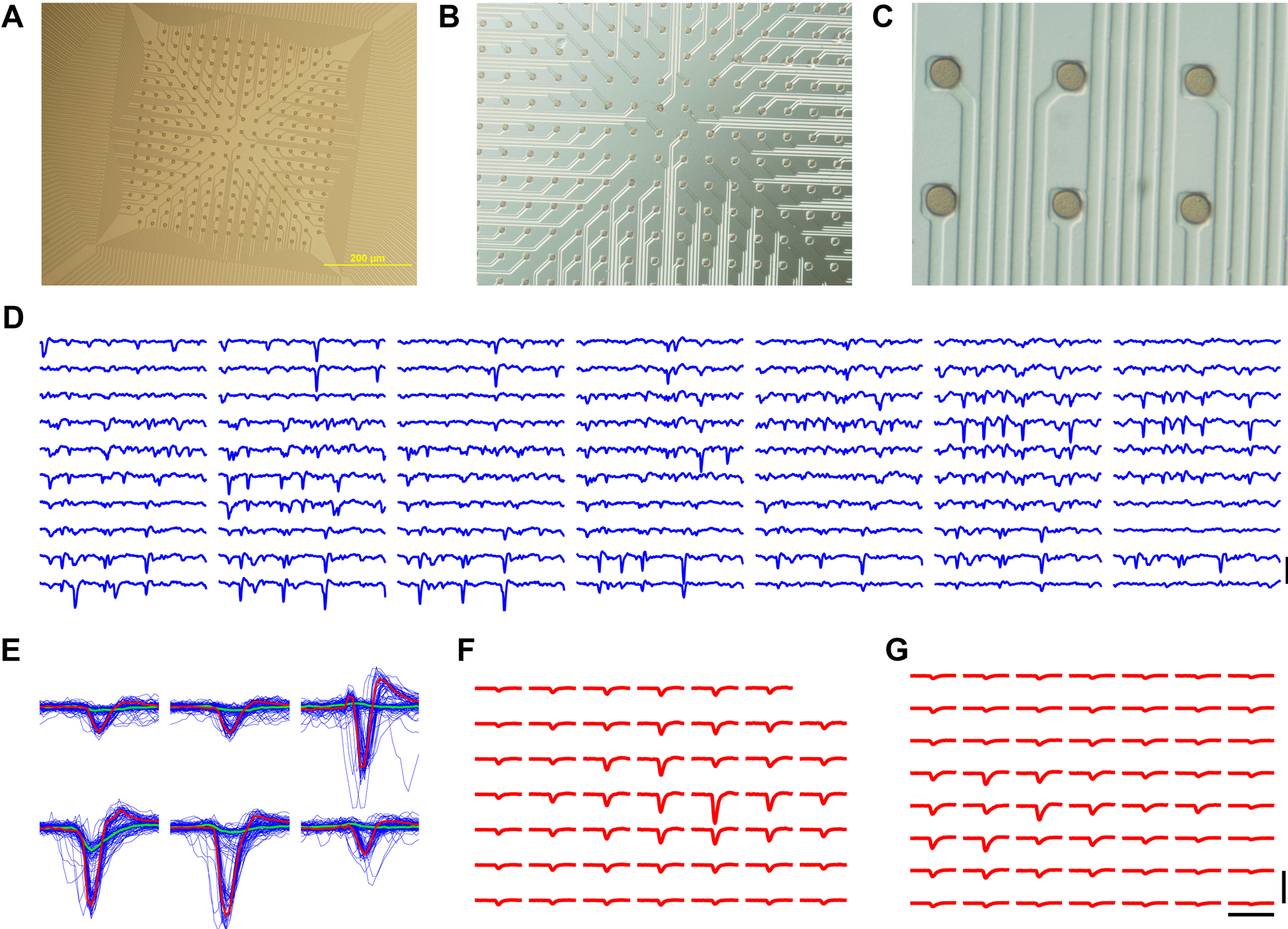
Example: Mouse in virtual reality
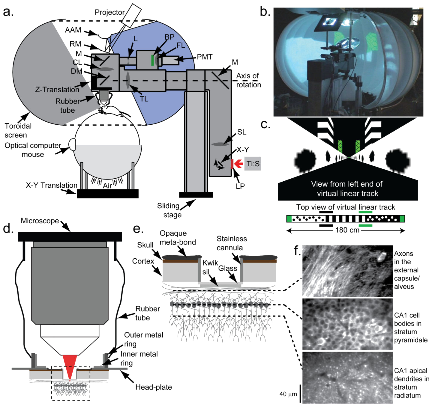
Mouse in a chamber
Dong Chuan Wu (吳東川)
China Medical University, Taichung
Problems with the data
- Large number of neurons
- Varying experimental conditions
- Non-specific neurons
Consider statistics (reduced dimensions) that are invariant under the selection of neurons, segmentation of signals, and the disturbance of the experimental conditions, while still carrying functionally relevant information.
- Characterize the network with model thermodynamics
- Extending the methodology to artificial network for machines of artificial intelligence
- Characterize the learning process with states of the networks
Idea of statistical modeling
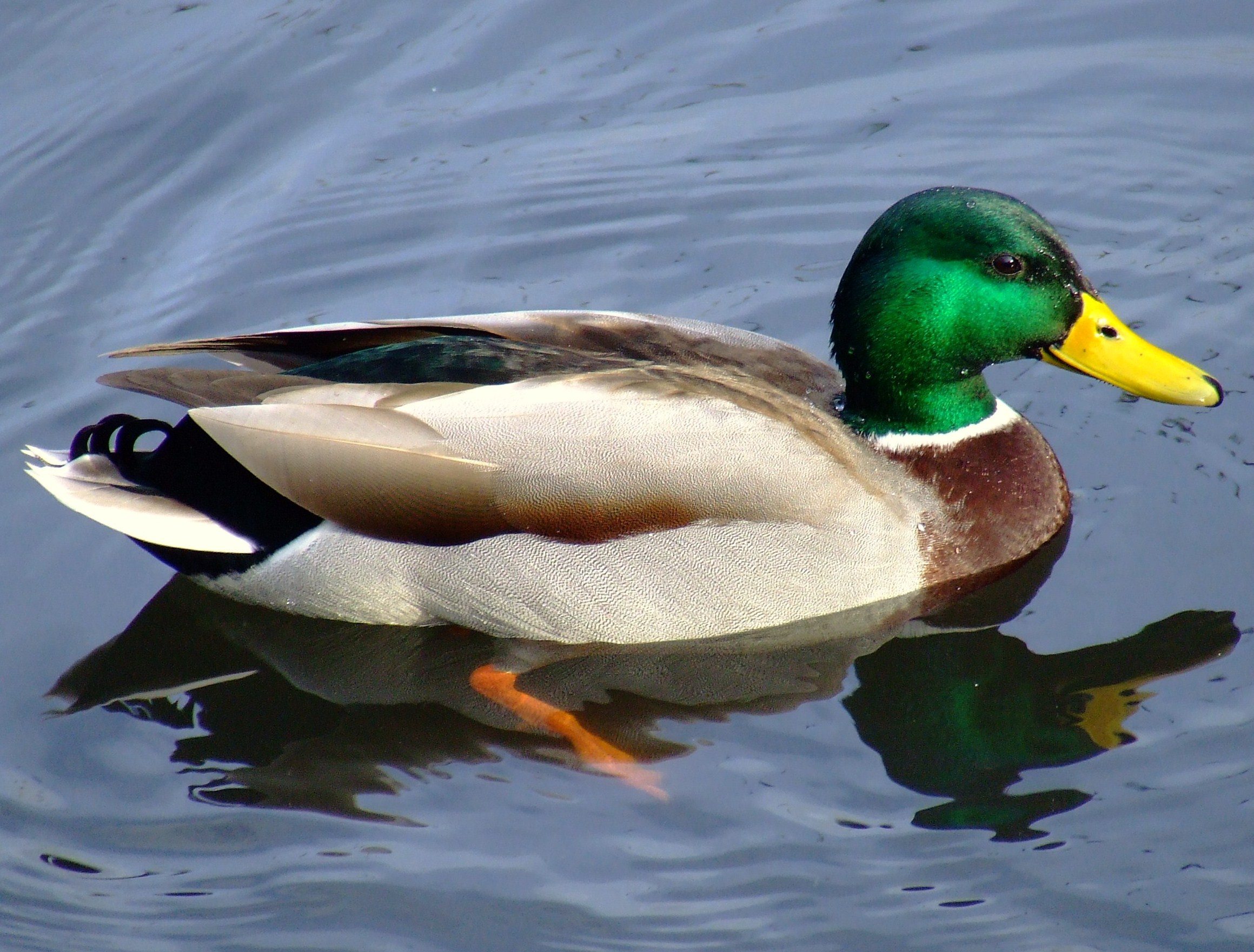
If it looks like a duck, swims like a duck, and quacks like a duck, then it probably is a duck it passes the duck's Turing test
Statistical properties
Data abstraction (segmentation)
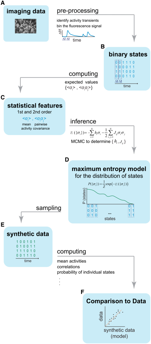
Spin-glass model for pair-wise interaction

Probability distribution of states is characterized by Hamiltonian
\[ \mathcal{H} = E = - \sum_i h_i s_i - \sum_{i,j} J_{i,j} s_i s_j \]
where spins \(s=\pm1\) represent possible variations of features in a state.

Model defined by \(h_i\) and \(J_{i,j}\)
Probability of a given state \(\left\{s_i\right\}\) is given by Boltzmann distribution\[P\left(\left\{s_i\right\}\right) = Z^{-1} \exp\left(-\beta E\right)\]
From spiking to spins

Spin-glass model \begin{eqnarray*}& E=-\sum_i h_i\sigma_i-\sum_{\langle i,j\rangle}J_{i,j}\sigma_i\sigma_j \\ & P\{\sigma_i\}\propto e^{-\beta E(\{s_i\})} \end{eqnarray*}
MCMC simulations
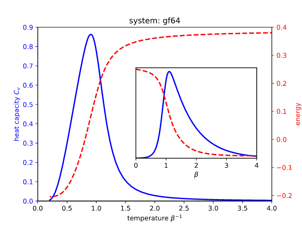
Thermodynamics
match properties
- Phase transition
- Criticality
- Scaling exponents
Critical state in neural networks
A common observation Natural systems are often poised near a critical state (peaks of $C_v$ found near $T=1$ in mapped models) See, for example,
- Mora & Bialek (2011) Are Biological Systems Poised at Criticality?
- Beggs & Timme (2012) Being Critical of Criticality in the Brain
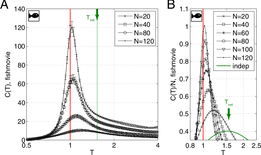
Ubiquitous proximity to a critical state
Chen et al. (2022) https://doi.org/10.1016/j.cjph.2021.12.010


Similar specific heat curves for various recordings and ways of segmentation...
Meanings of skewness and excess kurtosis

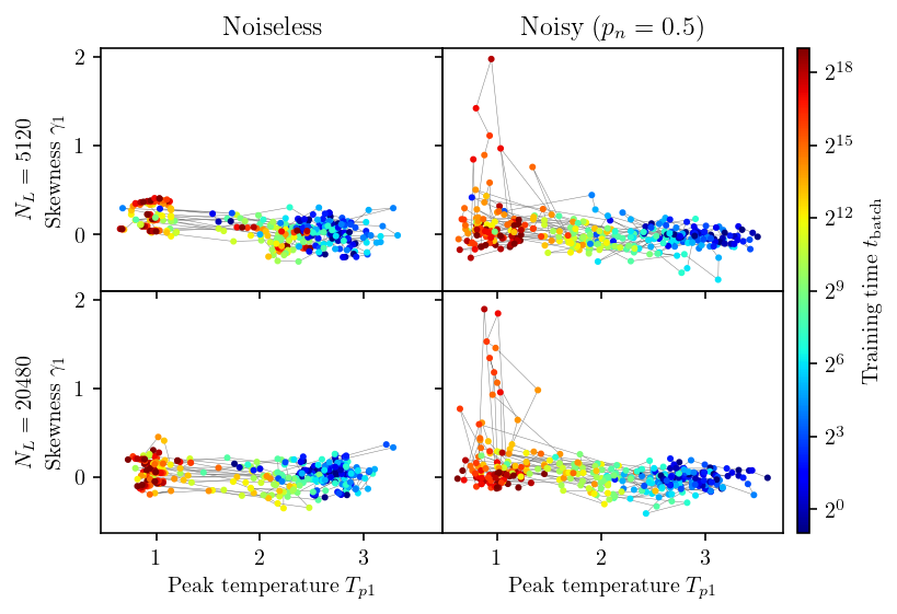
Skewness $\gamma_1 \equiv \langle (x_i - μ)^3\rangle/\sigma^3$ measures asymmetry.

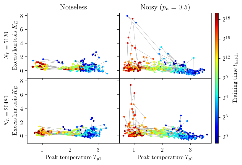
Kurtosis $K \equiv \langle (x_i - \mu)^4/\sigma^4\rangle$ measures the weight of tails.
Normal distribution $K = 3$, the excess kurtosis is defined as $$ K_E = K - 3. $$
More mouse experiment results (unpublished)


What have been learned
- Proximity to criticality (signaled by peak in specific heat vs temperature) is robust to sampling and segmentation
- Network structure is critical to the criticality
- Significant non-Gaussian long-tail on positive coupling strength observed in a fraction of the model networks
- All thresholds of coupling strengths result in networks with degree distribution consistent with Erdős–Rényi model
- How do the neural networks get to be near a critical state?
- Can we see the same proximity to a critical state in other networks?
Decoding the neural states of a brain


Application to artificial neural networks

MNIST dataset of handwritten digits

A typical architecture for solving MNIST

Dataset partitioning
Learning datasets are of sizes 320, 1280, 5120, and 20480 with equal number of sample images for each digits (‘0’…‘9’) chosen randomly from the original 60000 images of the MNIST training dataset. The rest of samples in the training dataset are used as the testing dataset to verify the existence of over training.
Making harder for the machines
An independent Gaussian noise is added to each pixel of an input image.


Training process under noise

Apply statistical modeling to internal states

Treating the internal nodes just as neurons in animal brains
☆ Similar to protocol for biological neurons, the outputs of the nodes are binarized using it's STD as the threshold.
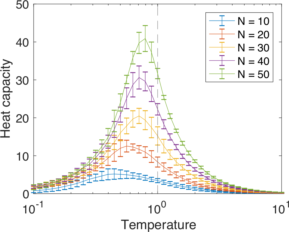
Evolution of specific heat curves
Noise influences specific heat curves

Peak shift signifies change in thermodynamic properties of the model in the learning processes, with which the network approaches criticality $T_{p1}\rightarrow 1$But, what happened to the network structure and states?
Coupling strength $J_{i,j}$ distribution

Coupling strength distribution developes significant long-tail for noisy cases when networks are optimally trained: Some links are significantly stronger than others, and likely effecting the functional dynamics of the networks
The skewness and criticality
The excess kurtosis and criticality
Activation probabilities of internal nodes

Activation probabilities of nodes show non-monotonic variation over the training. Without noise, activation levels after the network is optimally trained. With noise, activation keeps decreasing after a peak activation until the end of our run.
Entropy of internal state distribution
Take $\beta$ derivative of the Helmholtz free energy $$ F\equiv U - TS = - T\ln Z $$ we find $\frac{\partial S}{\partial U} = \beta$. The energy—temperature curve, or $\beta(U)$, can be integrated from infinite temperature, $\beta = 0$, to find entropy $$ S(\beta) = S(0) + \int_{U(0)}^{U(\beta)} \beta(U) dU $$ Since all states are equally likely at $\beta=0$, the entropy is given by $S(0) = N\ln 2$.
☆ Numerical calculations in the high temperature regime are generally more stable since there are less meta-stable states to trap the simulation dynamics.
Entropy of the internal nodes

A minimum of entropy occurs around the activation peak of internal nodes before the networks are optimally trained. How are these related to the functional behavior of the networks?
Explainable artificial intelligence
→ Can be justified as a form of deep-Taylor decomposition
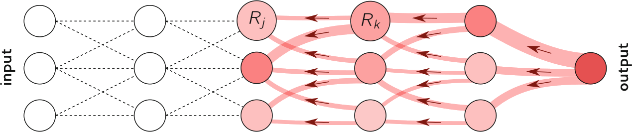
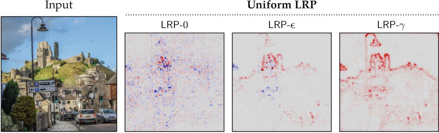
Apply LRP to the machines

Evolution of relevance map
Quantify the clarity of relevance heat map
Variance of the heat map pixels $R(x)$ $$ \frac{(\sum_x R(x)-\bar{R})^2}{N_\mathrm{px}} $$ where $\bar{R} = \sum_x R(x)/N_\mathrm{px}$, $N_\mathrm{px}$ is the number of pixel.
Mean square local gradient of the heat map $$\left|\frac{\partial R(x)}{\partial x} \right|^2 $$
☆ Both are calculated and averaged over the pixel locations $x$.
Contrast and sharpness

☆ Shaded area represents standard deviation across the test data set.
Compare with entropy & magnetization
Conclusion 1/2
- Statistical modeling can extract information from large volume of neural data that is robust to selection of neurons and details of segmentation
- Thermodynamics of the mapped models exhibit peaked specific heat that can separate the phase space into different regions
- Training process in ANN results in shift and morphology change of the specific heat curves that are also influenced by different training conditions and tends to bring the network towards a critical state
Conclusion 2/2
- For the MNIST recognizing network, training is seen fall into an earlier stage with decreasing entropy of network states and increasing contrast of relevance heat map and a later stage with increasing entropy and decreasing contrast.
- The two stages are separated by a local peak in the activation level of the neurons or the magnetization of the model spins.