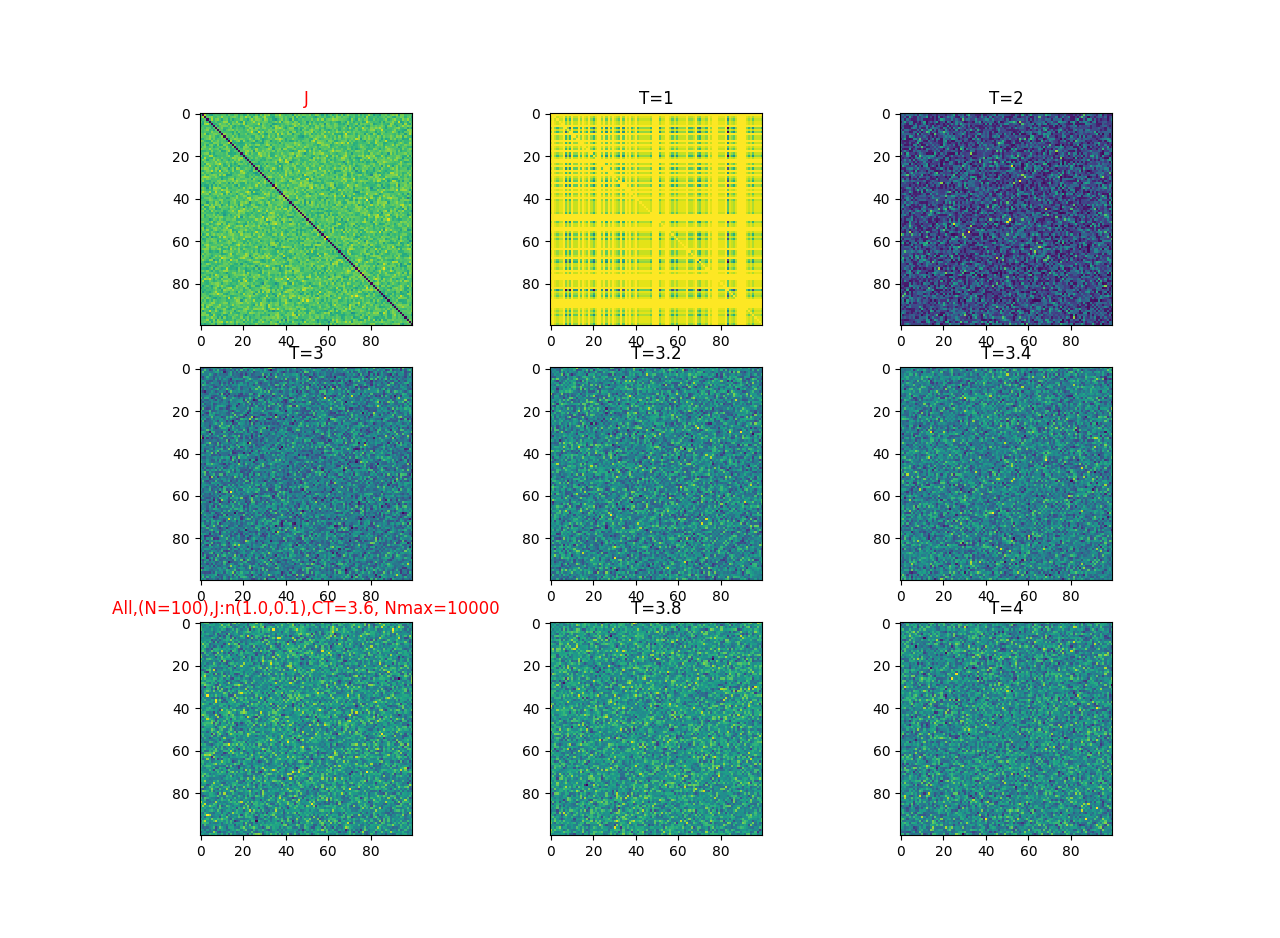
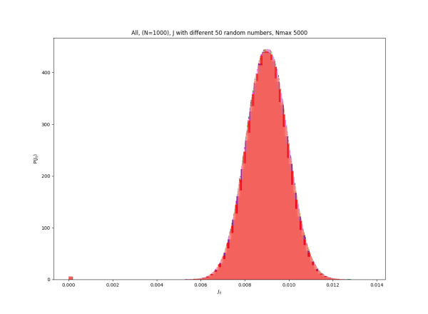
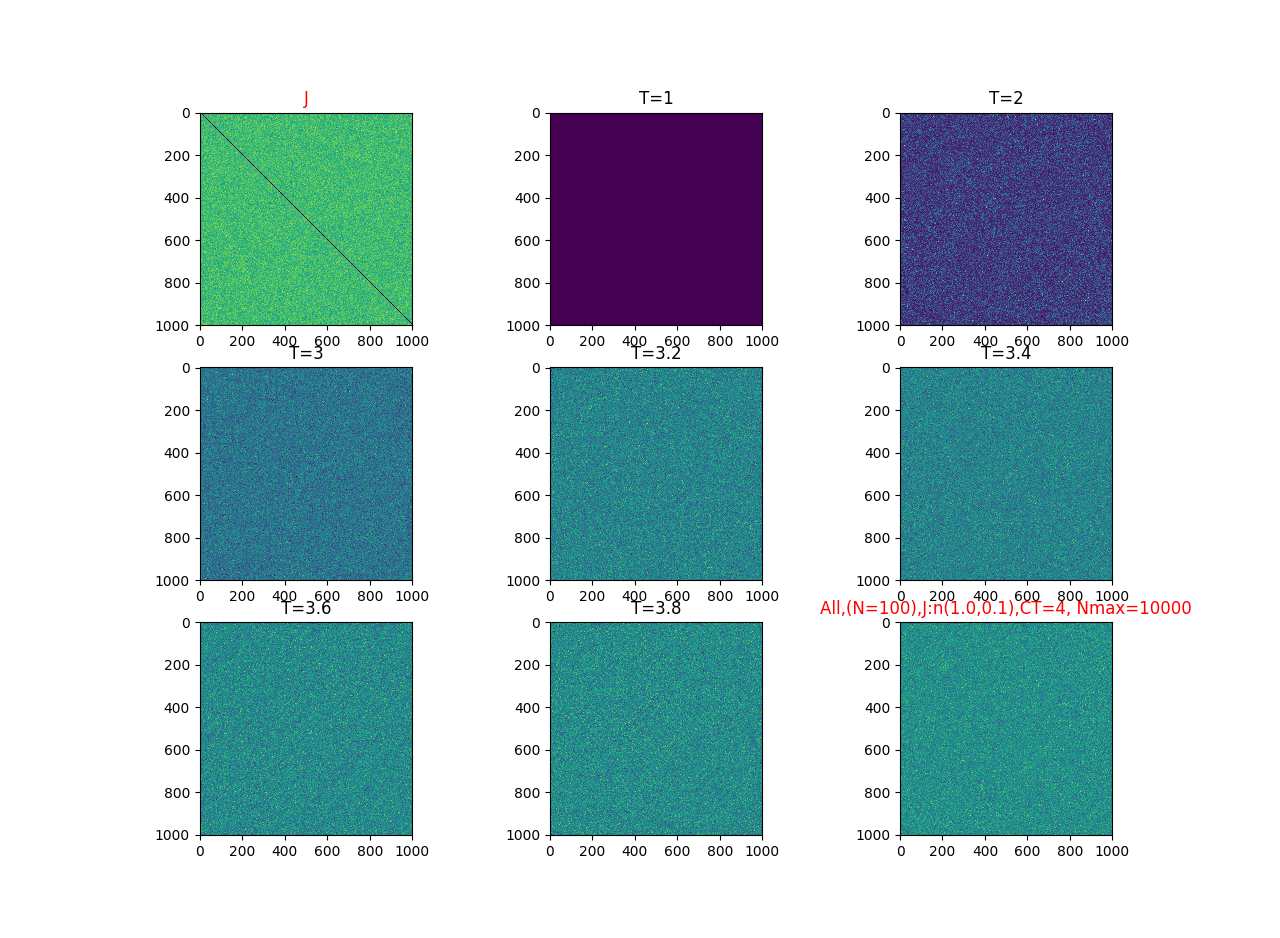
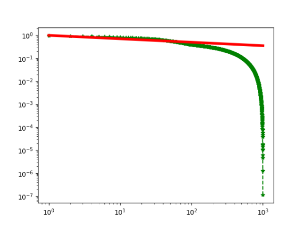
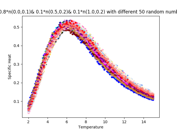
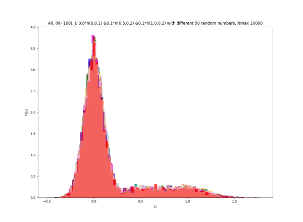
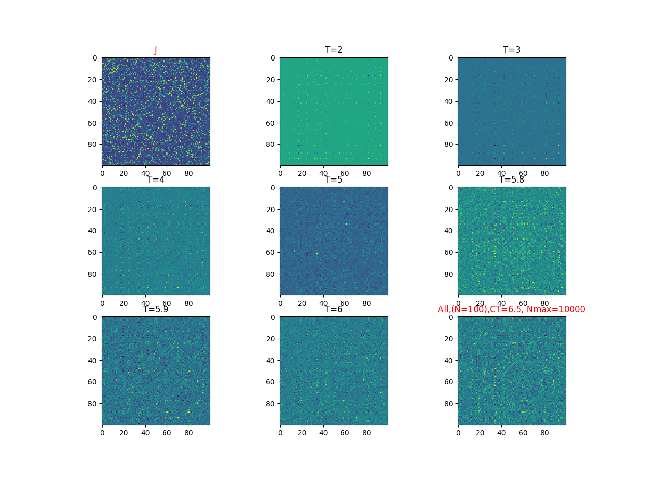
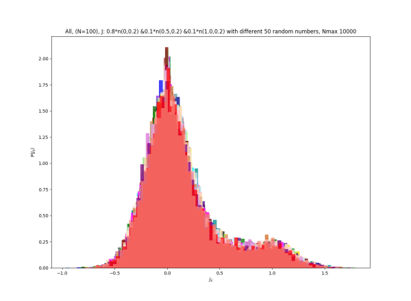
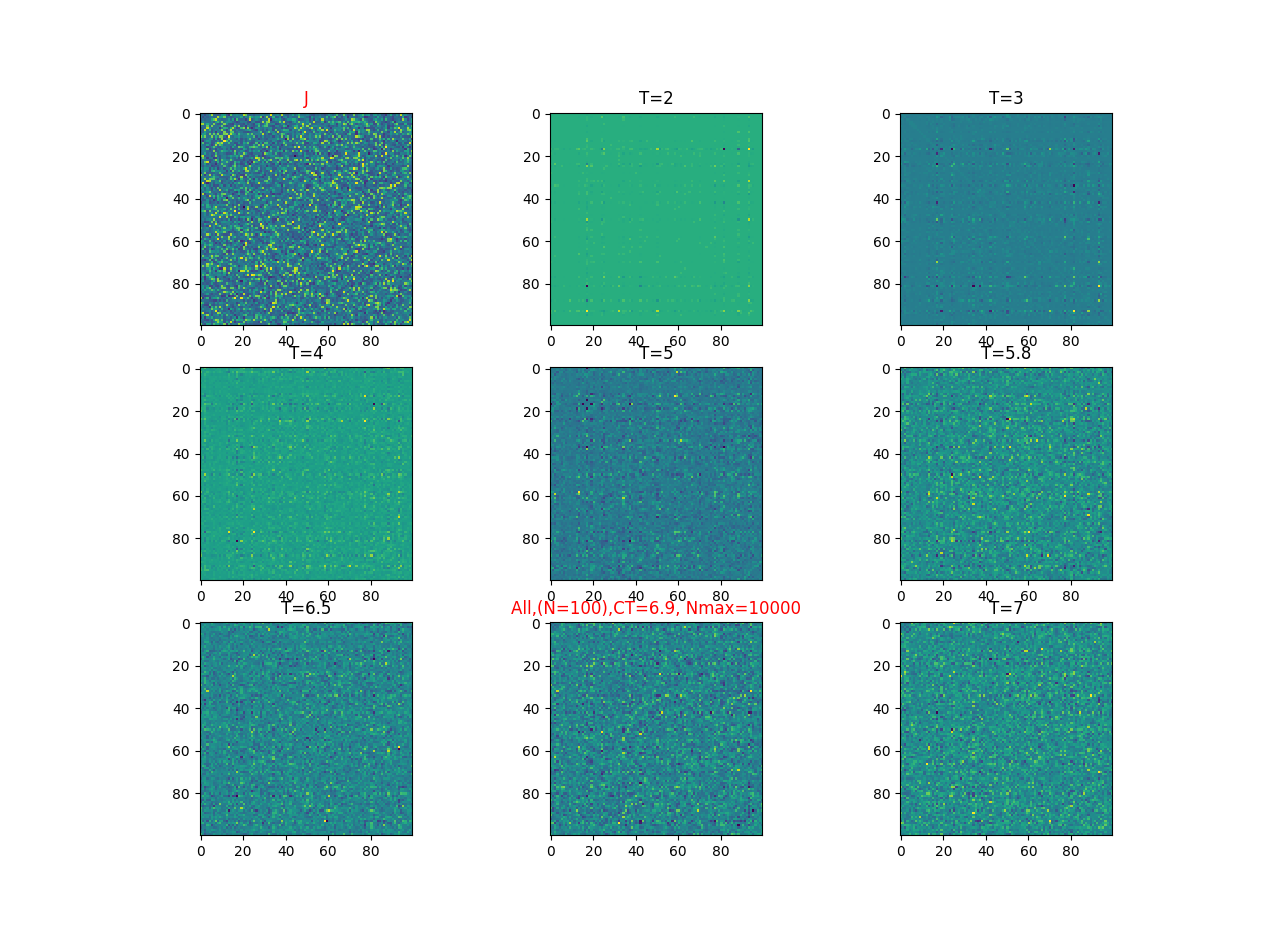
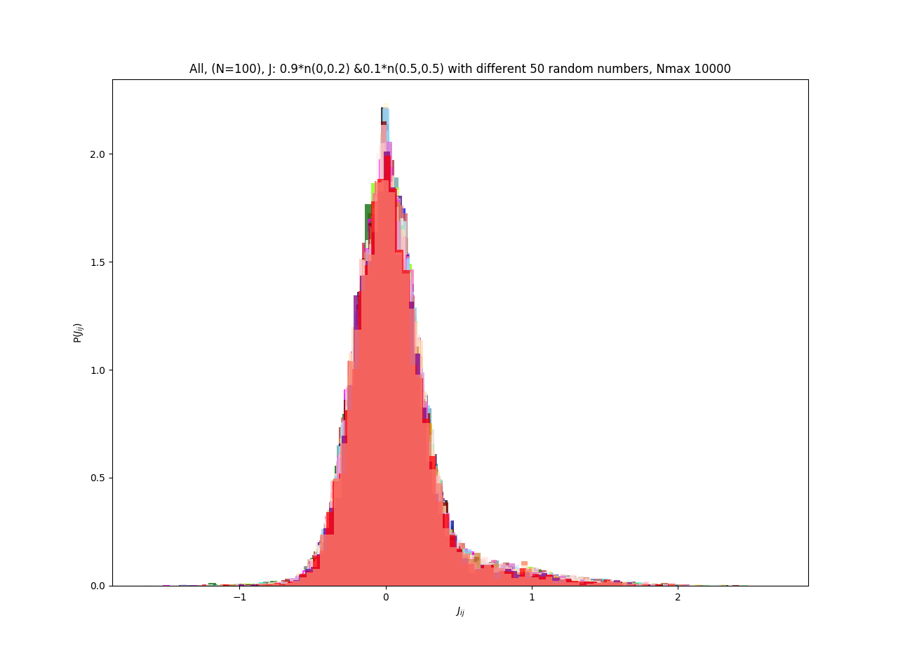
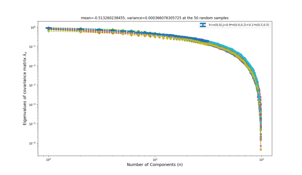
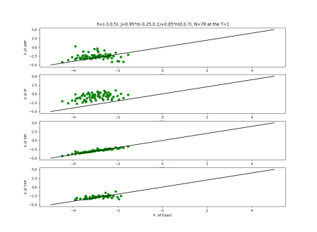
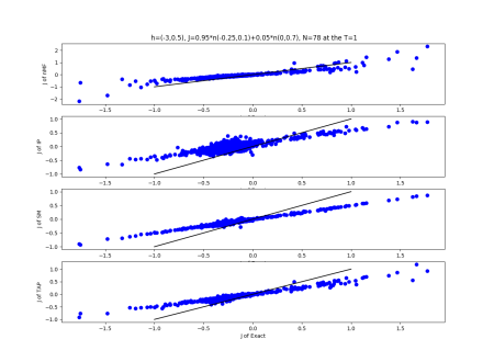
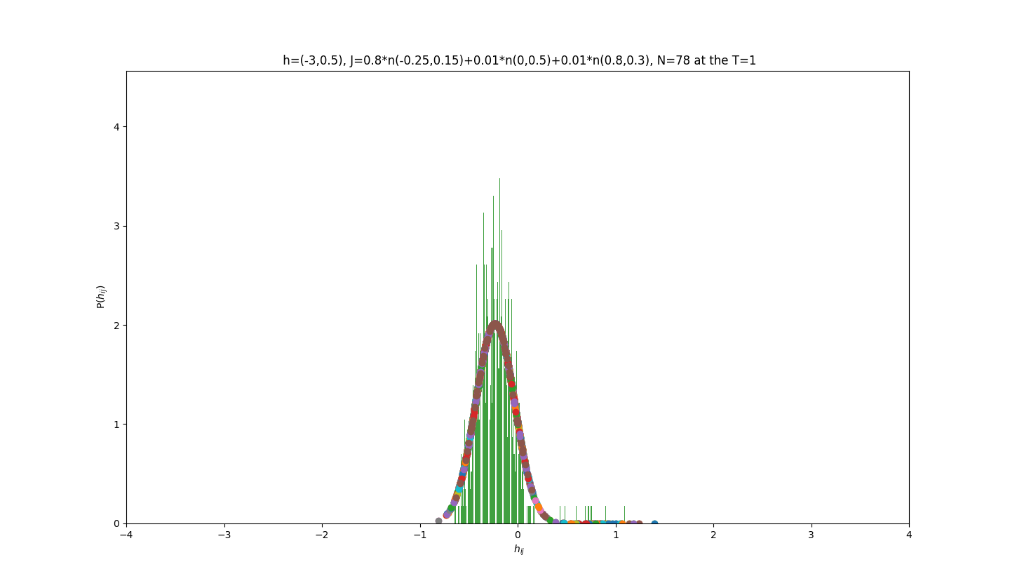
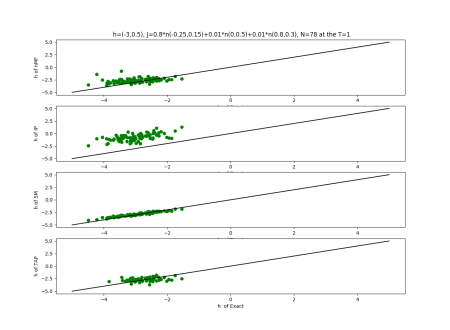
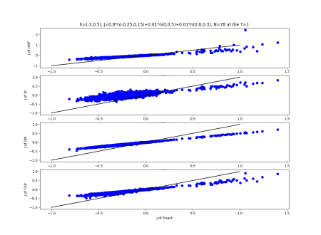
2019-09-16 :Case N1: long tail antiferromagentic
2018-07-2 :The solutions to the inverse Ising problem
Method: Boltzmann learning
Finding the external fields $h_{i}$ and the coupling parameters $J_{ij}$ can fit the same means and pairwise covariance as the experiment data, using the equations
$\left<s_{i}\right>_{Ising} = \left<s_{i}\right>_{data} $
$\left<s_{i}s_{j}\right>_{Ising} = \left<s_{i}s_{j}\right>_{data} $.
We can solve the equations by iterations $h_{i}=h_{i}+\delta h_{i}$ and $J_{ij}=J_{ij}+\delta J_{ij}$ then make changes
$\delta h_{i}=\eta \{\left<s_{i}\right>_{data} - \left<s_{i}\right>_{Ising} \} $
$\delta J_{ij}=\eta \{\left<s_{i}s_{j}\right>_{data} - \left<s_{i}s_{j}\right>_{Ising} \} $.
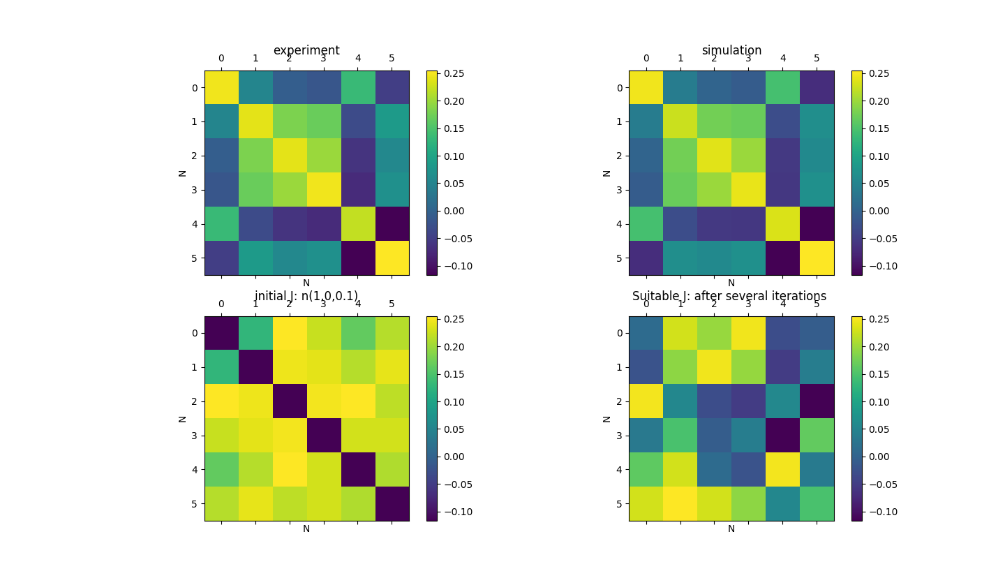
We use the data ACV_slice5 (6 neurons) as our sample and set $\eta = 0.1$.
The cost function is
${(\left<s_{i}\right>_{data} - \left<s_{i}\right>_{Ising})}^{2} \leq 0.00000001$
&&
${(\left<s_{i}s_{j}\right>_{data} - \left<s_{i}s_{j}\right>_{Ising})}^{2} \leq 0.00000001$.
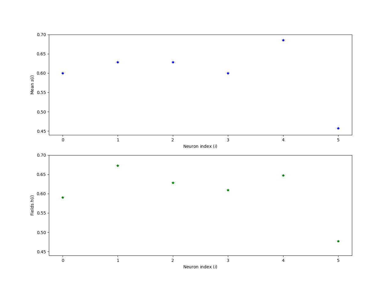
The experiment result and simulation result see figure.
| Mean $s_{i}$ | 0.600000 | 0.628571 | 0.628571 | 0.600000 | 0.685714 | 0.457143 |
| Simulation $s_{i}$ | 0.590619 | 0.672644 | 0.628609 | 0.609595 | 0.647693 | 0.477471 |


If the number of neurons is larger than 30, it is very slow to find the suitable $h_{i}$ and $J_{ij}$ for the good fitting.
2018-07-2 :The solutions to the inverse Ising problem
7.2.18
7.2.18
2018-07-9 :The solutions to the inverse Ising problem
7.10.18
| | mean | variance |
| J: 1*n(0.0,0.1) | -0.789370 | 0.001288 |
| J: 1*n(0.0,0.2) | -0.914673 | 0.003162 |
| J: 1*n(0.0,0.3) | -0.901516 | 0.002877 |
| J: 0.9*n(0.0,0.1)+0.1*n(0.5,0.5) | -0.412155 | 0.000304 |
| J: 0.9*n(0.0,0.2)+0.1*n(0.5,0.5) | -0.513260 | 0.000366 |
| J: 0.9*n(0.0,0.3)+0.1*n(0.5,0.5) | -0.532969 | 0.000416 |
| J: 0.8*n(0.0,0.1)+0.1*n(0.5,0.2)+0.1*n(1,0.2) | -0.356512 | 0.000270 |
| J: 0.8*n(0.0,0.2)+0.1*n(0.5,0.2)+0.1*n(1,0.2) | -0.370494 | 0.000255 |
| J: 0.8*n(0.0,0.3)+0.1*n(0.5,0.2)+0.1*n(1,0.2) | -0.393506 | 0.000367 |
| J: 0.9*n(0.0,0.1)+0.1*n(-0.5,0.5) | -1.287893 | 0.003625 |
| J: 0.9*n(0.0,0.2)+0.1*n(-0.5,0.5) | -1.215945 | 0.004903 |
| J: 0.9*n(0.0,0.3)+0.1*n(-0.5,0.5) | -1.166773 | 0.003841 |


7.19.18 Inverse Problem
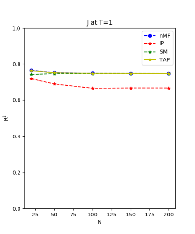
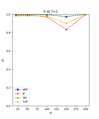
The coefficient of $R^{2}$ is:
$R^{2}=1-\frac{\sum_{ij} \left(J_{ij}^{\text{approx}}-J_{ij}^{\text{Exact}} \right)^{2} }{\sum_{ij} \left(J_{ij}^{\text{Exact}}-J_{ij}^{\text{$\overline{Exact}$}} \right)^{2}}$ ,
with
$\overline{J_{ij}^{\text{Exact}}}=\frac {\sum_{i \neq j} J_{ij}^{\text{Exact}}}{N(N-1)}$.
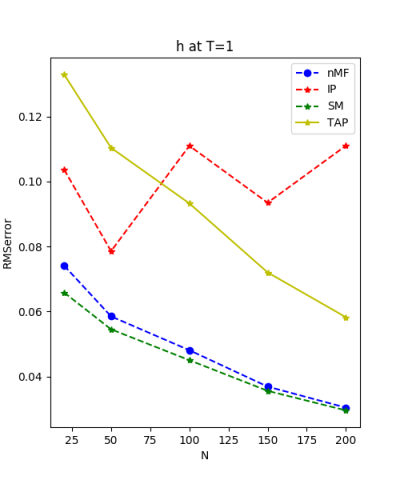
The rms error is:
$\sqrt{\frac{1}{N(N-1)} \sum_{i \neq j} (J_{ij}^\text{approx}-J_{ij}^\text{Exact})^{2} }$.
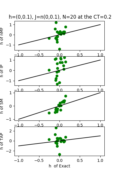
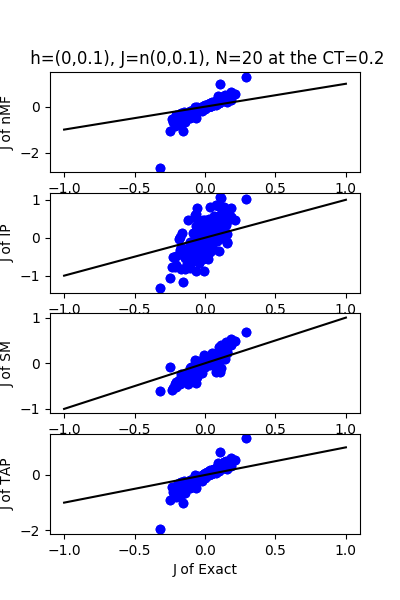
| h:n(0.0,0.1)&J:n(0.0,0.1) , n=20 at CT=0.2 | rms error | $R^{2}$ |
| nMf | 0.261099 | -5.69658 |
| IP | 0.36969 | -12.4251 |
| SM | 0.135638 | -0.807203 |
| TAP | 0.225045 | -3.97488 |


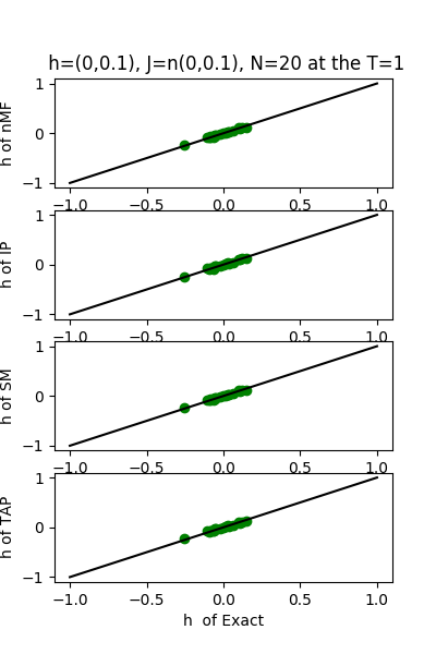
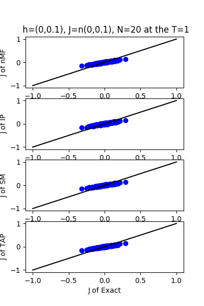
| h:n(0.0,0.1)&J:n(0.0,0.1) ,n=20 at T=1 | rms error | $R^{2}$ |
| nMf | 0.0501364 | 0.753083 |
| IP | 0.0492352 | 0.761881 |
| SM | 0.0504632 | 0.749854 |
| TAP | 0.0501487 | 0.752963 |


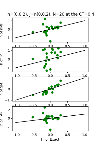
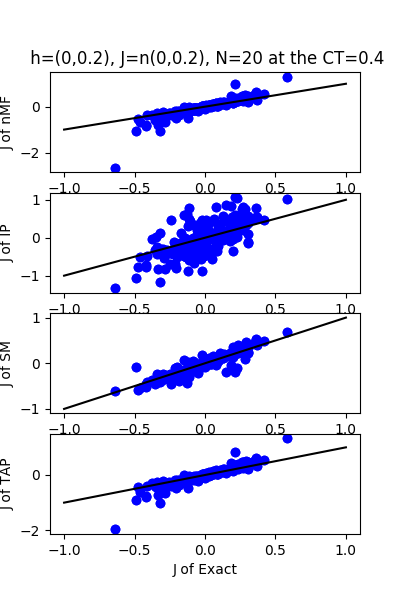
| h:n(0.0,0.2)&J:n(0.0,0.2) ,n=20 at CT=0.4 | rms error | $R^{2}$ |
| nMf | 0.186599 | 0.144925 |
| IP | 0.327701 | -1.63717 |
| SM | 0.0808463 | 0.83949 |
| TAP | 0.146637 | 0.471956 |


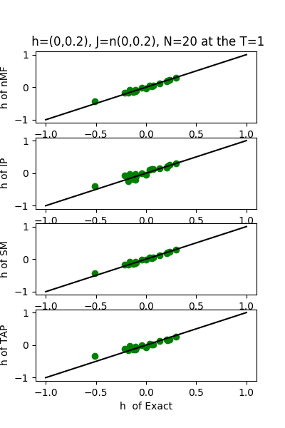
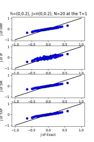
| h:n(0.0,0.2)&J:n(0.0,0.2) ,n=20 at T=1.0 | rms error | $R^{2}$ |
| nMf | 0.0989592 | 0.759511 |
| IP | 0.105152 | 0.72847 |
| SM | 0.102435 | 0.74232 |
| TAP | 0.0992857 | 0.757921 |


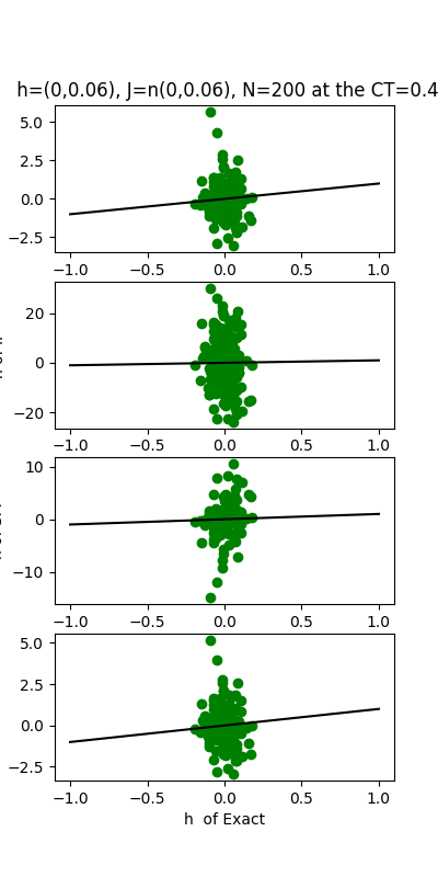
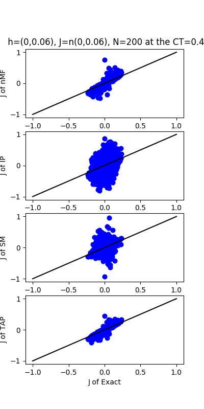
| J:n(0.0,0.06) ,n=200 at T=0.4 | rms error | $R^{2}$ | h:n(0.0,0.06) | rms error | $R^{2}$ |
| nMf | 0.0252805 | 0.820135 | | 1.40724 | -0.111763 |
| IP | 0.135993 | -4.20489 | | 14.1081 | -110.741 |
| SM | 0.0429129 | 0.481737 | | 3.8296 | -7.23352 |
| TAP | 0.021821 | 0.865994 | | 1.48845 | -0.243794 |


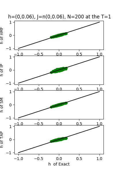
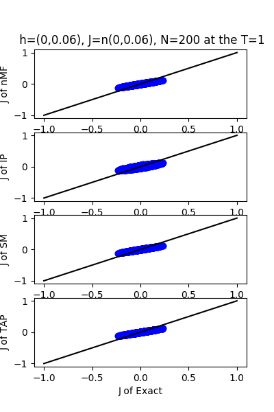
| J:n(0.0,0.06) ,n=200 at T=1.0 | rms error | $R^{2}$ | h:n(0.0,0.06) | rms error | $R^{2}$ |
| nMf | 0.0299218 | 0.748029 | | 0.0187765 | 0.999802 |
| IP | 0.033059 | 0.692421 | | 0.0524186 | 0.998457 |
| SM | 0.0299849 | 0.746966 | | 0.0184704 | 0.999808 |
| TAP | 0.0299236 | 0.747998 | | 0.0354793 | 0.999293 |


7.24.18 Inverse Problem
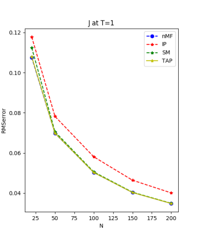
| h:n(0.0,0.07) & J:n(0.0,0.07), n=200 at T=1 | $\sqrt{200}$ |
| h:n(0.0,0.08) & J:n(0.0,0.08), n=150 at T=1 | $\sqrt{150}$ |
| h:n(0.0,0.1) & J:n(0.0,0.1) , n=100 at T=1 | $\sqrt{100}$ |
| h:n(0.0,0.14) & J:n(0.0,0.14), n=50 at T=1 | $\sqrt{50} $ |
| h:n(0.0,0.22) & J:n(0.0,0.22), n=20 at T=1 | $\sqrt{20} $ |
We set the mean equal to zero and the variance of normal distribution of h and J
from $\frac{1}{\sqrt{200}}$: $\frac{1}{\sqrt{150}}$: $\frac{1}{\sqrt{100}}$:$\frac{1}{\sqrt{50}}$:$\frac{1}{\sqrt{20}} \approx 0.07 : 0.08 : 0.1 : 0.14 : 0.22 $.
We use the normal distribution of h and J to get the coefficients of $R^{2}$ and the RMSerror at T=1.


7.24.18 Inverse Problem data
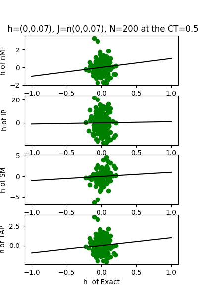
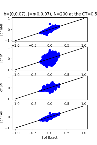
| J:n(0.0,0.07) ,n=200 at CT=0.5 | rms error | $R^{2}$ | h:n(0.0,0.07) | rms error | $R^{2}$ |
| nMf | 0.0123978 | 0.968219 | | 0.884148 | 0.67757 |
| IP | 0.117457 | -1.85258 | | 10.4116 | -43.7117 |
| SM | 0.0227896 | 0.892612 | | 1.57309 | -0.0206929 |
| TAP | 0.0107151 | 0.97626 | | 1.11072 | 0.491141 |


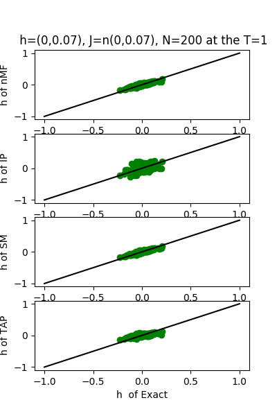
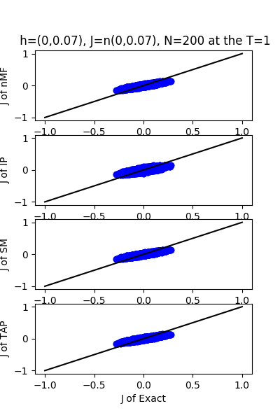
| J:n(0.0,0.07) ,n=200 at T=1.0 | rms error | $R^{2}$ | h:n(0.0,0.07) | rms error | $R^{2}$ |
| nMf | 0.0348459 | 0.748936 | | 0.0304221 | 0.999618 |
| IP | 0.0401123 | 0.667312 | | 0.110992 | 0.994919 |
| SM | 0.0349555 | 0.747353 | | 0.0295671 | 0.999639 |
| TAP | 0.0348501 | 0.748876 | | 0.0582334 | 0.998601 |


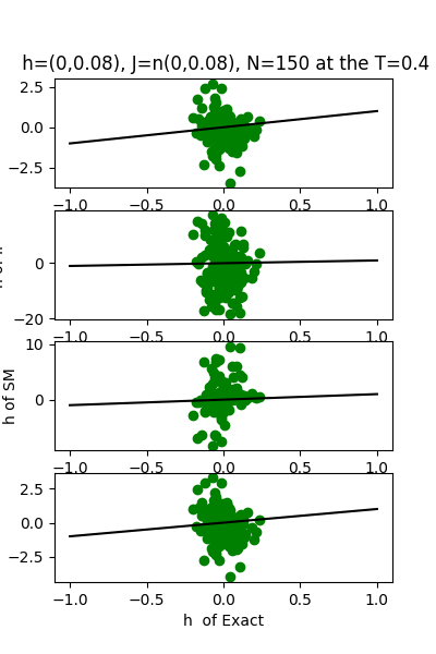
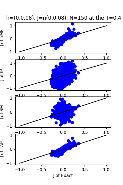
| J:n(0.0,0.08) ,n=150 at CT=0.4 | rms error | $R^{2}$ | h:n(0.0,0.08) | rms error | $R^{2}$ |
| nMf | 0.0389121 | 0.766413 | | 1.28183 | -30.3925 |
| IP | 0.240864 | -7.94997 | | 12.1312 | -2810.72 |
| SM | 0.0757059 | 0.115825 | | 3.75663 | -268.628 |
| TAP | 0.0338997 | 0.822715 | | 1.67608 | -52.6732 |


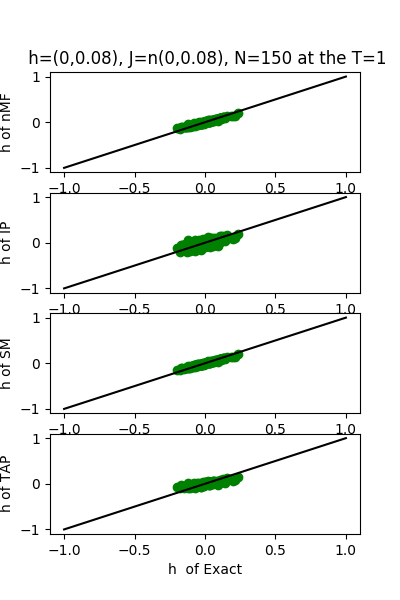
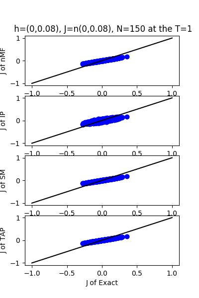
| J:n(0.0,0.08) ,n=150 at T=1 | rms error | $R^{2}$ | h:n(0.0,0.08) | rms error | $R^{2}$ |
| nMf | 0.0403046 | 0.749396 | | 0.0368884 | 0.974002 |
| IP | 0.0464303 | 0.667431 | | 0.0934541 | 0.833136 |
| SM | 0.0404719 | 0.747311 | | 0.0355802 | 0.975813 |
| TAP | 0.0403135 | 0.749285 | | 0.0720108 | 0.900926 |


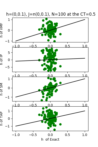
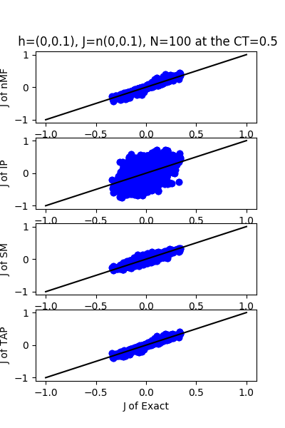
| J:n(0.0,0.1) ,n=100 at CT=0.5 | rms error | $R^{2}$ | h:n(0.0,0.1) | rms error | $R^{2}$ |
| nMf | 0.0182768 | 0.96695 | | 0.596538 | 0.18199 |
| IP | 0.200247 | -2.96735 | | 6.28192 | -89.7127 |
| SM | 0.0280065 | 0.922396 | | 0.603074 | 0.163966 |
| TAP | 0.0164129 | 0.973348 | | 0.89636 | -0.846922 |


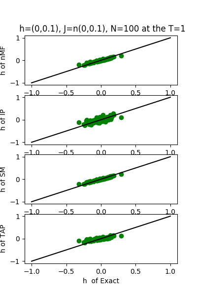
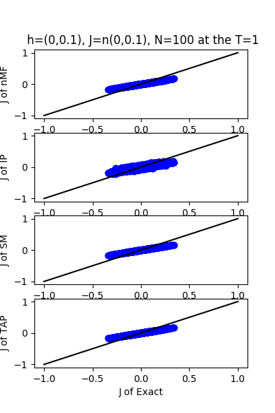
| J:n(0.0,0.1) ,n=100 at T=1 | rms error | $R^{2}$ | h:n(0.0,0.1) | rms error | $R^{2}$ |
| nMf | 0.0502492 | 0.750181 | | 0.0480846 | 0.994685 |
| IP | 0.0581101 | 0.665905 | | 0.110959 | 0.971698 |
| SM | 0.0505891 | 0.74679 | | 0.0450164 | 0.995342 |
| TAP | 0.0502829 | 0.749846 | | 0.0932494 | 0.980012 |


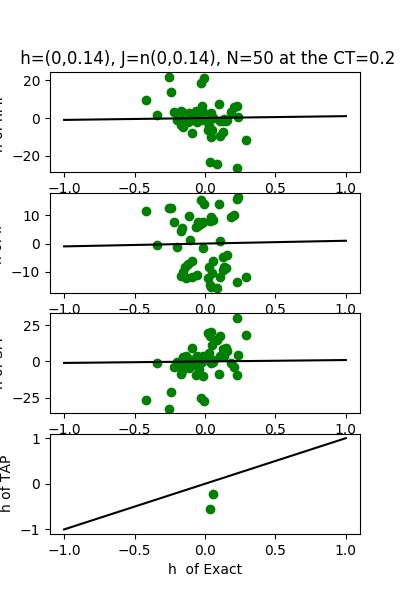
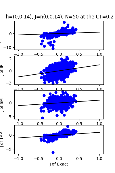
| J:n(0.0,0.14) ,n=50 at CT=0.2 | rms error | $R^{2}$ | h:n(0.0,0.14) | rms error | $R^{2}$ |
| nMf | 0.331738 | -50.2182 | | 7.59468 | -77.9424 |
| IP | 0.200528 | -17.7147 | | 8.27031 | -92.6128 |
| SM | 0.276861 | -34.6743 | | 10.0695 | -137.774 |
| TAP | 0.0472849 | -0.0405847 | | 0.12614 | 0.978223 |


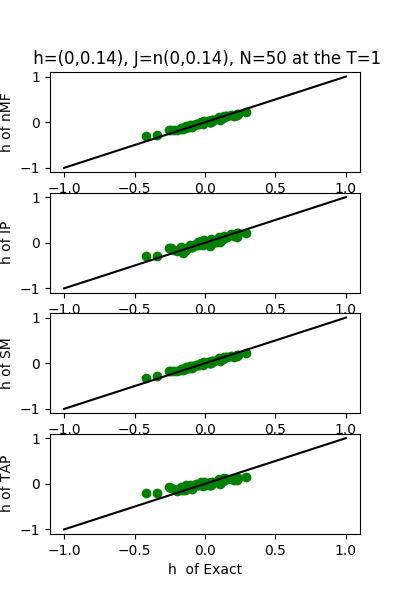
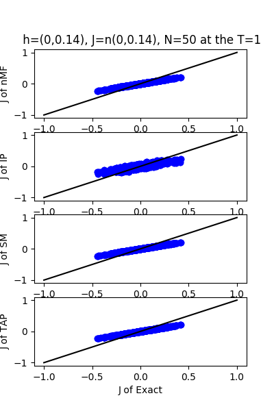
| J:n(0.0,0.14) ,n=50 at T=1 | rms error | $R^{2}$ | h:n(0.0,0.14) | rms error | $R^{2}$ |
| nMf | 0.0697652 | 0.753093 | | 0.0584891 | 0.995397 |
| IP | 0.0781925 | 0.689839 | | 0.0785585 | 0.991696 |
| SM | 0.0705361 | 0.747606 | | 0.054511 | 0.996002 |
| TAP | 0.0698489 | 0.752499 | | 0.110346 | 0.983615 |


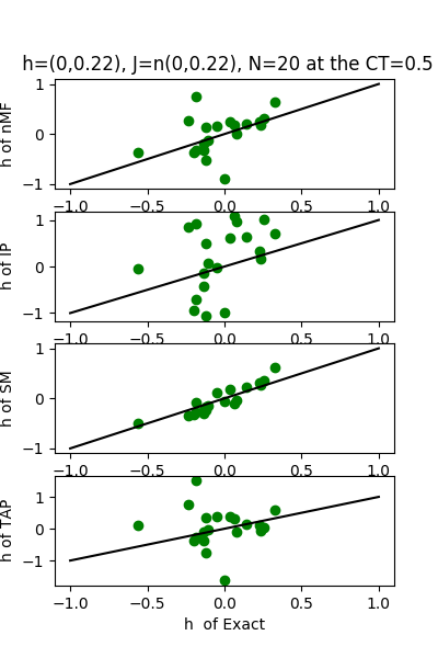
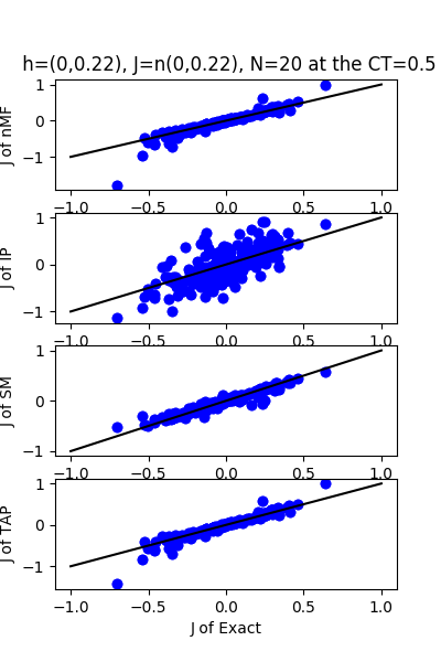
| J:n(0.0,0.22) ,n=20 at CT=0.5 | rms error | $R^{2}$ | h:n(0.0,0.22) | rms error | $R^{2}$ |
| nMf | 0.107295 | 0.766355 | | 0.495427 | 0.715343 |
| IP | 0.264862 | -0.423761 | | 0.946502 | -0.0389783 |
| SM | 0.0572563 | 0.933466 | | 0.177233 | 0.963571 |
| TAP | 0.0846797 | 0.854469 | | 0.910756 | 0.0380179 |


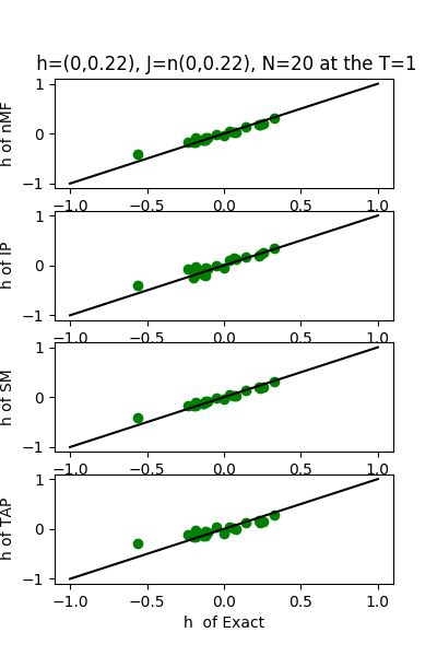
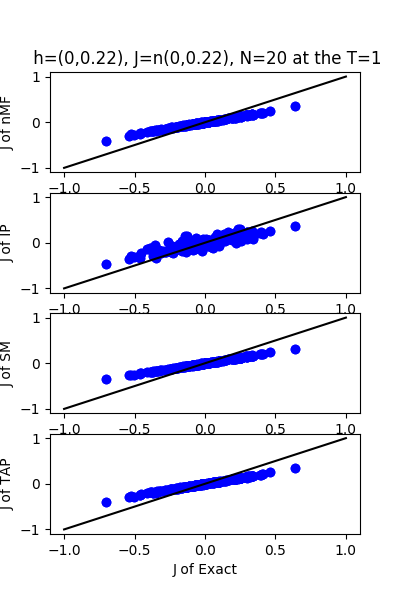
| J:n(0.0,0.22) ,n=20 at T=1 | rms error | $R^{2}$ | h:n(0.0,0.22) | rms error | $R^{2}$ |
| nMf | 0.107456 | 0.765655 | | 0.0741133 | 0.99363 |
| IP | 0.117774 | 0.718488 | | 0.103663 | 0.987537 |
| SM | 0.112377 | 0.743699 | | 0.0658366 | 0.994973 |
| TAP | 0.10791 | 0.763667 | | 0.132923 | 0.979509 |


7.30.18 Inverse Problem data

